

![]()
![]()
![]()
![]()
Text in early stages - needs tidying and content
De
Forest one day sucked the air out of an old glass bulb one day. It had just been
laying around and had a two terminal filament of wire with another piece of
metal placed next to it. He connected the filament wires to a battery and
watched the cosy dull red glow from its metal wire filament. Then he thought
about that forgotten third terminal – why not connect that to a battery also
and see what would happen. To his surprise, actually it made no difference –
the filament glowed pretty much the same – but then he placed his ammeter in
the current path to the third terminal.
What
De Forest found was a slight twitch on the dial – how, he asked in silence of
his lab, could current travel those cold empty distances of space? The third
terminal was not connected, and a vacuum separated it from the filament. But
when the filament glowed, De Forest could see the ammeter needle twitch.

Although
I was not there at the time, I guess De Forest must have felt some sense of
adventure in all of this. For some reason the hot metal filament was releasing
electrons into the local vacuum and these were being attracted to the third
electrode that carried a positive, attracting charge. In this way a small but
measurable electric current flowed from the negative battery terminal, launched
itself into the vacuum of space inside De Forest’s glass bulb, got collected
by the third terminal which had a positive attracting bias and then flowed back
through De Forest’s ammeter to the battery’s positive terminal.
In
those small quiet moments De Forest grasped the implications alone and imagined
what if the filament was hotter, or if more positive voltage was available to
attract even more electrons. Or even, what if the polarity was reversed –
would those pesky electrons be repelled by the negative charge on that third
terminal and be sent hurtling safely back home?
De
Forest tried a crack at all of this, and the vacuum diode was born.
Soon
everyone wanted one of these devices. The vacuum diode became a “one way”
device, i.e. it would pass current in one direction but block it in another.
This allowed it to convert alternating current “AC” signal into direct
current “DC” signals. In two particular ways this invention was timely,
| The
1920’s etc had adopted AC power for house-by-house distribution. This was
fine for light bulbs and allowed convenient voltage transformation, but how
could people charge up that old Henry Ford motor-car battery when it went
flat? AC was no good, but if a vacuum diode could covert it to DC then
people could be off to a racing start | |
| AM
Broadcast had just begun – at first primitive spark gaps but more was soon
to follow. The vacuum diode was the first jump-start to technology into the
land of amplification and oscillation.
|
Hence
the good old vacuum “diode” came into focus in our history at a very
convenient time.
People
had been playing around with static electricity even before the time of the
Egyptians. Sparks seen and felt when rubbing a cat’s fur were commonplace.
They had all done the two “orange pith” on a string trick, watching them
stay apart when static electricity was around. The repulsive nature of electrons
were evident even to them, so why put them into commodity product’s like the
then day vacuum tube?
I
guess the simple answer is that when there’s gold in them darn hills, why then
someone’s got to mine it. Could a diode be made to do more than just rectify
– could static repulsion be used to make it return a mother-load from even
small incoming signals. At this point perhaps a short diversion is justified,
The ocean going ships of the time had very little way to communicate situations of distress and call for rescue when needed. The most they could do is play semaphore games to people back on land if they could be seen, or make loud fog horn calls if they could be heard. However people such as Nikola Tesla had been experimenting with coils that make high voltage discharges, and wanted to send power throughout the world based on resonant transmission line effects between the planets surface and its atmosphere. Marconi wanted to do the same but on a smaller scale. His interest was to make a big spark in one local wire loop recreate a smaller spark in another remote wire loop. His experiments sparked a revolution. The birth of radio communication screamed with flashes of light, the smell of ozone and loud crackling noises.
What Marconi showed was that information, not just power, could be transmitted at a distance “over the air”. Just as those electrons in De Forest’s vacuum diode did soon to follow. So what if a big boat had some massive big spark generator – surely a remote person monitoring could see some tiny flash if trouble came and raise an alarm? Well sadly no. The sparks fading too quickly with distance and the second remote antenna couldn’t outreach the semaphore eye.
Some people thought about this and reasoned that the distance of the receiving spark gap was the problem. Perhaps there are transactions on this subject? How could the gap be made smaller so that the tiny sparks could fly across and make their mark?
I forget who the bright spark was but someone came up with the idea of filling a glass tube with rusting old iron filings. Either she or he attached electrodes to each end. When a RF pulse came along some of the filings would arc and short, allowing a DC current to pass.
|

The simple mechanical “coherer” evolved with self resetting versions but never would have the ability to recover speech transmissions. Morse Code was its domain and it was firmly there to stay. Or so it thought – until De Forest’s vacuum diode came along.
Soon after the diode came the triode and the poor coherer was quickly doomed.
The
coherer was simple and cheap, but lacked sensitivity and always needed a good
tapping. The vacuum diode was far more effective in detecting RF signals and was
self resetting to boot. However it was still “deaf” by today’s standards
and needed something to boost the signal prior to rectification. Further the
maritime spark generator transmitters seriously polluted the RF spectrum and
people sought to see them banned in favour of a cleaner signal source. This is
were the triode valve sought is first entry point – its electrons could be
controlled by static charges and currents could be made to follow the
application of voltage

At
the time this was a remarkable discovery. Since the grid was negatively charged
it drew no current as the electrons were repelled by it. This hindered, and
eventually could prevent them from reaching the positively charged Anode.
Consequently almost zero power was required to control the Anode current. Since
this was able to operate at a very high Anode voltage, the potential so
generating significant power variation in a load resistance from an
infinitesimal Grid control signal power quickly lit the imagination of many.
Finally the amplification device that people had long dreamt for had arrived.
Two
subsequent pioneers, Hartley and Collpitts soon discovered that the vacuum
triode could be used to generate continuous sinusoidal output signals. Their
“oscillators” consisted of a vacuum triode, a resonant tuned feedback
circuit and a DC supply. Unlike the broad output spectrum produced by maritime
spark gap transmitters, these oscillators produced a pure single frequency tone.
They, and others experimented with many variations on the same theme, and soon
high power, clean signal sources were available. Now that many people could
occupy the same common spectrum at different transmit frequencies, the use of
spark gap transmitters was soon outlawed.
Despite the magnificent break-though performance of
the vacuum triode it was not without its limitations. Even given improvements in
vacuum technology that allowed anode voltages up to ~3000 V to be supported, it
was still an inefficient amplifier. The effect of the grid voltage on electron
flow was also influenced by anode voltage. High Anode voltages attracted more
electrons from the Cathode filament and increased the Grid voltage needed to
stop their flow. This form of “internal negative feedback” reduced the
amount of voltage gain that the early vacuum triode could achieve. In addition,
even Grid voltages of –zero volts could only support a finite Anode current,
and this Anode current reduced as the Anode voltage fell. This restricted the
maximum Anode voltage output swing, and so DC to signal output power was
compromised.
At one stage in the vacuum triode history, people
began to experiment with positive grid voltage control. Although grid current
was drawn and input drive power was increased, useful power gain was still
possible and output efficiency gains were obtained. The positive grid voltage
attracted electrons, far more so than would otherwise have reached the Anode.
These new tubes promised to be the solution.
Such positive grid control devices emerged for a
short time until the penny dropped – why not place this positive attracting
field on a separate grid? The main control grid could then remain negatively
charged and so draw no current. This second “screen grid” could draw the
electrons forward and hurtle them towards the Anode. More importantly, once pass
the Screen Grid the Anode voltage would capture them as effectively with low
Anode voltage as with high.
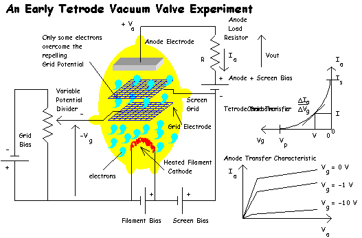
A second unexpected improvement resulted. The close
proximity between Grid and Anode in the vacuum triode resulted in significant
Grid-Anode feedback capacitance. In the early AM Tuned Radio Frequency (TRF)
broadcast receivers, several valves were successively lined up to amplify weak
incoming signals. In order to achieve high power amplification and selectivity,
high impedance resonant coupling circuits were needed. However the internal
feedback capacitance of the triode resulted in self-oscillation. Some
compensating “neutralising” circuits were needed, requiring delicate
adjustment at each received frequency. The Tetrode however placed an isolating
“screen grid” between the two terminals, and the several pF coupling seen in
the vacuum Triode was reduced to less than 0.02 pF.
However even these improvements did not come at a
cost. The vacuum Tetrode suffered from an effect called “secondary
emission”. At certain low Anode voltages the screen grid appeared positive to
its lower potential and attracted electrons from it. The electrical consequence
was a region of negative resistance in the Anode voltage versus current transfer
curve, leading to audio distortion and the potential for instability at large
output voltage excursions.
A simple solution was soon found. These unwanted
Anode electrons could be re-attracted by the inclusion of a third grid between
the Screen grid 1 and the Anode. This Screen grid 2 was kept at zero potential
and the resulting 5-terminal structure was called the vacuum Pentode.
As
previously mentioned, early AM broadcast radios used TRF technology, in which
multiple RF amplifying stages were cascaded up the point of RF to Audio AM
demodulation. Each of these RF stages used tracking RF tuned circuits to pass a
wanted signal frequency and reject others.
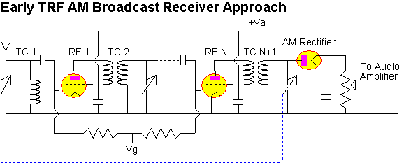
This
approach was very much in vogue by the early 1930’s, but required much skill
in tuning, especially as “ganged” multiple sets of tuning capacitors were
not readily available and each tuned circuit had to be simultaneously tuned to a
given radio station for it to be heard. In earlier vacuum Triode designs,
additional “neutralisation” trimmers had to also be adjusted for each RF
stage to retain stability. Consequently, once set up, people seldom ventured to
the misery of changing to another radio channel.
|
Because
the technology relating to oscillators had been previously established (Hartley
and Collpitts), some people wondered if these could not be used somehow in a
receiver. After all, people were very familiar with the audio beat note, or
howl, that arose from a mistuned AM broadcast receiver. Only Armstrong had the
mad genius to connect the observation with improvements to receiver design. He
made use of the non linear properties of amplifiers to convert energy from one
part of the radio spectrum to another.
Armstrong
found that if a valve amplifier was supplied with a weak RF input signal, and if
an additional large amplitude sine wave was also applied, then the valve would
create outputs at sum and difference frequencies. This realisation was to be the
champion idea behind almost all current receiver (and some transmitter)
architectures.

Armstrong
called these new frequencies “Intermediate Frequencies” or IF. Several
important advantages were evident.
| The
receive frequency could be adjusted by tuning just one oscillator circuit | |
| A
single RF input tuned circuit was sufficient to reject one of the
“image” frequencies
| |
| All
main amplification could occur at a single fixed IF frequency | |
| Gain
at Low frequencies was much easier to obtain than gain at RF | |
| Frequency
selectivity was also easier to obtain with fixed, low frequency IF’s |
This,
to Armstrong, was the best thing since sliced bread, and he knew he had a
winner. This superhet technology made VHF and UHF reception possible, and
inexpensive. Only two high frequency devices were needed to process RF,
everything else could work down at much lower, and easy to process frequencies.
Still, some drawbacks existed. The method of introducing the LO signal required
a common electrode, and this not only caused oscillator loading (and frequency
pulling) effects, but also allowed a sizable LO signal to leak out to the
antenna, causing potential interference to other spectrum users. Armstrong
needed a better mixer device.
Various
configurations were tried, ranging from injecting the LO signal into the
Cathode, or Screen grid 1 and even Screen grid 2. All three methods gave good
results and the combination of Screen grid 1 as a “virtual Anode” and the
Cathode even allowed a simple oscillator to be constructed inside the mixing
valve. However such configurations were never optimum in terms of convenience.
Soon
people trigged that the LO signal could be injected into any of the valve’s
grid terminals, and that sum and difference frequencies would be generated, they
began to see the process of frequency conversion as a multiplication function.
Voltage on one grid could control the gain of the device to a signal on a
different grid. This quickly led to the generation of a special mixer valve
called a Hexode (6 terminals) and Heptode (7 terminals).
These
new mixer valves used control grid 1 for RF signal input and the “suppresser
grid 3) for LO injection. A forth grid was also added after grid 3 to further
attract electrons by adding additional positive charge. However the ugly head of
“secondary emission” reared once more, so a 5th suppressor grid
was added, connected to ground. This completed the final evolution in valve
mixer technology, or so it seemed.
All
mixer structures so far were single ended or “un balanced”. For simple
receivers this was fine, but what if maximum dynamic range was needed. A push
pull or “balanced” approach could at least add superior even order mixer
term rejection. In the early low density RF environment non linear effects in
valves was somewhat unimportant, but as the number of transmitters increased,
and their signal powers, “spurious responses” in the mixing process started
to become a big concern.
As
mentioned previously, sum and difference frequencies are generated by the mixing
process. However products relating to combinations of RF and LO harmonics also
occur. These allow unwanted frequencies to be received in places where they
should not be.
For
example, let’s say we want to receive an AM radio station at 1.4 MHz using an
IF frequency of 500 kHz. We could use an LO frequency of 1.9 MHz or 0.9 MHz.
Let’s choose this higher option. The second harmonic of the LO signal is 3.8
MHz, and the third harmonic of an incoming RF signal at 1.4333.. MHz is 4.3 MHz.
This combination will produce the same IF output frequency of 0.5 MHz. A signal
as close as 33.3.. kHz from the wanted signal could elicit a spurious response!
A
few solutions were proposed – all based on the idea of push pull topologies
that could provide second order cancellation. One particular mixer tube had two
Anodes whose electron streams where switched by between them by a common but
inverted LO signal. But by now the semiconductor revolution had begun, and the
dinosaur cult of the valve was poised to a break point of imminent failure.
![]()
Return to: A Component Universe
or: Ian Scotts Technology Pages
© Ian R Scott 2007 - 2008